What is KNN Algorithm?
K nearest neighbors or KNN Algorithm is a simple algorithm which uses the entire dataset in its training phase. Whenever a prediction is required for an unseen data instance, it searches through the entire training dataset for k-most similar instances and the data with the most similar instance is finally returned as the prediction.
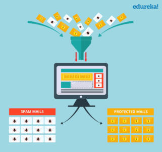
kNN is often used in search applications where you are looking for similar items, like find items similar to this one.
Algorithm suggests that if you’re similar to your neighbours, then you are one of them. For example, if apple looks more similar to peach, pear, and cherry (fruits) than monkey, cat or a rat (animals), then most likely apple is a fruit.
How does a KNN Algorithm work?
The k-nearest neighbors algorithm uses a very simple approach to perform classification. When tested with a new example, it looks through the training data and finds the k training examples that are closest to the new example. It then assigns the most common class label (among those k-training examples) to the test example.
KNN Algorithm using Python | Edureka
Subscribe to our YouTube channel to stay updated with our fresh content

What does ‘k’ in kNN Algorithm represent?
k in kNN algorithm represents the number of nearest neighbor points which are voting for the new test data’s class.
If k=1, then test examples are given the same label as the closest example in the training set.
If k=3, the labels of the three closest classes are checked and the most common (i.e., occurring at least twice) label is assigned, and so on for larger ks.
kNN Algorithm Manual Implementation
Let’s consider this example,
Suppose we have height and weight and its corresponding Tshirt size of several customers. Your task is to predict the T-shirt size of Anna, whose height is 161cm and her weight is 61kg.

Step1: Calculate the Euclidean distance between the new point and the existing points
For example, Euclidean distance between point P1(1,1) and P2(5,4) is:


Step 2: Choose the value of K and select K neighbors closet to the new point.
In this case, select the top 5 parameters having least Euclidean distance

Step 3: Count the votes of all the K neighbors / Predicting Values
Since for K = 5, we have 4 Tshirts of size M, therefore according to the kNN Algorithm, Anna of height 161 cm and weight, 61kg will fit into a Tshirt of size M.

Implementation of kNN Algorithm using Python
-
Handling the data
-
Calculate the distance
-
Find k nearest point
-
Predict the class
- Check the accuracy
Don’t just read it, practise it!
Step 1: Handling the data
The very first step will be handling the iris dataset. Open the dataset using the open function and read the data lines with the reader function available under the csv module.
import csv
with open(r'C:\Users\Atul Harsha\Documents\iris.data.txt') as csvfile:
	lines = csv.reader(csvfile)
	for row in lines:
		print (', '.join(row))
Now you need to split the data into a training dataset (for making the prediction) and a testing dataset (for evaluating the accuracy of the model).
Before you continue, convert the flower measures loaded as strings to numbers. Next, randomly split the dataset into train and test dataset. Generally, a standard ratio of 67/33 is used for test/train split
Adding it all, let’s define a function handleDataset which will load the CSV when provided with the exact filename and splits it randomly into train and test datasets using the provided split ratio.
import csv
import random
def handleDataset(filename, split, trainingSet=[] , testSet=[]):
	with open(filename, 'r') as csvfile:
	    lines = csv.reader(csvfile)
	    dataset = list(lines)
	    for x in range(len(dataset)-1):
	        for y in range(4):
	            dataset[x][y] = float(dataset[x][y])
	        if random.random() < split:
	            trainingSet.append(dataset[x])
	        else:
	            testSet.append(dataset[x])
Let’s check the above function and see if it is working fine,
Testing handleDataset function
trainingSet=[]
testSet=[]
handleDataset(r'iris.data.', 0.66, trainingSet, testSet)
print ('Train: ' + repr(len(trainingSet)))
print ('Test: ' + repr(len(testSet)))
Step 2: Calculate the distance
In order to make any predictions, you have to calculate the distance between the new point and the existing points, as you will be needing k closest points.
In this case for calculating the distance, we will use the Euclidean distance. This is defined as the square root of the sum of the squared differences between the two arrays of numbers
Specifically, we need only first 4 attributes(features) for distance calculation as the last attribute is a class label. So for one of the approach is to limit the Euclidean distance to a fixed length, thereby ignoring the final dimension.
Summing it up let’s define euclideanDistance function as follows:
import math
def euclideanDistance(instance1, instance2, length):
	distance = 0
	for x in range(length):
		distance += pow((instance1[x] - instance2[x]), 2)
	return math.sqrt(distance)
Testing the euclideanDistance function,
data1 = [2, 2, 2, 'a']
data2 = [4, 4, 4, 'b']
distance = euclideanDistance(data1, data2, 3)
print ('Distance: ' + repr(distance))
Step 3: Find k nearest point
Now that you have calculated the distance from each point, we can use it collect the k most similar points/instances for the given test data/instance.
This is a straightforward process: Calculate the distance wrt all the instance and select the subset having the smallest Euclidean distance.
Let’s create a getKNeighbors function that returns k most similar neighbors from the training set for a given test instance
import operator
def getKNeighbors(trainingSet, testInstance, k):
	distances = []
	length = len(testInstance)-1
	for x in range(len(trainingSet)):
		dist = euclideanDistance(testInstance, trainingSet[x], length)
		distances.append((trainingSet[x], dist))
	distances.sort(key=operator.itemgetter(1))
	neighbors = []
	for x in range(k):
		neighbors.append(distances[x][0])
	return neighbors
Testing getKNeighbors function
trainSet = [[2, 2, 2, 'a'], [4, 4, 4, 'b']]
testInstance = [5, 5, 5]
k = 1
neighbors = getNeighbors(trainSet, testInstance, 1)
print(neighbors)
Step 4: Predict the class
Now that you have the k nearest points/neighbors for the given test instance, the next task is to predicted response based on those neighbors
You can do this by allowing each neighbor to vote for their class attribute, and take the majority vote as the prediction.
Let’s create a getResponse function for getting the majority voted response from a number of neighbors.
import operator
def getResponse(neighbors):
	classVotes = {}
	for x in range(len(neighbors)):
		response = neighbors[x][-1]
		if response in classVotes:
			classVotes[response] += 1
		else:
			classVotes[response] = 1
	sortedVotes = sorted(classVotes.items(), key=operator.itemgetter(1), reverse=True)
	return sortedVotes[0][0]
Testing getResponse function
neighbors = [[1,1,1,'a'], [2,2,2,'a'], [3,3,3,'b']]
print(getResponse(neighbors))
Step 5: Check the accuracy
Now that we have all of the pieces of the kNN algorithm in place. Let’s check how accurate our prediction is!
An easy way to evaluate the accuracy of the model is to calculate a ratio of the total correct predictions out of all predictions made.
Let’s create a getAccuracy function which sums the total correct predictions and returns the accuracy as a percentage of correct classifications.
def getAccuracy(testSet, predictions):
	correct = 0
	for x in range(len(testSet)):
		if testSet[x][-1] is predictions[x]:
			correct += 1
	return (correct/float(len(testSet))) * 100.0
Testing getAccuracy function
testSet = [[1,1,1,'a'], [2,2,2,'a'], [3,3,3,'b']]
predictions = ['a', 'a', 'a']
accuracy = getAccuracy(testSet, predictions)
print(accuracy)
Since we have created all the pieces of the KNN algorithm, let’s tie them up using the main function.
# Example of kNN implemented from Scratch in Python
import csv
import random
import math
import operator
def handleDataset(filename, split, trainingSet=[] , testSet=[]):
with open(filename, 'rb') as csvfile:
lines = csv.reader(csvfile)
dataset = list(lines)
for x in range(len(dataset)-1):
for y in range(4):
dataset[x][y] = float(dataset[x][y])
if random.random() < split: trainingSet.append(dataset[x]) else: testSet.append(dataset[x]) def euclideanDistance(instance1, instance2, length): distance = 0 for x in range(length): distance += pow((instance1[x] - instance2[x]), 2) return math.sqrt(distance) def getNeighbors(trainingSet, testInstance, k): distances = [] length = len(testInstance)-1 for x in range(len(trainingSet)): dist = euclideanDistance(testInstance, trainingSet[x], length) distances.append((trainingSet[x], dist)) distances.sort(key=operator.itemgetter(1)) neighbors = [] for x in range(k): neighbors.append(distances[x][0]) return neighbors def getResponse(neighbors): classVotes = {} for x in range(len(neighbors)): response = neighbors[x][-1] if response in classVotes: classVotes[response] += 1 else: classVotes[response] = 1 sortedVotes = sorted(classVotes.iteritems(), key=operator.itemgetter(1), reverse=True) return sortedVotes[0][0] def getAccuracy(testSet, predictions): correct = 0 for x in range(len(testSet)): if testSet[x][-1] == predictions[x]: correct += 1 return (correct/float(len(testSet))) * 100.0 def main(): # prepare data trainingSet=[] testSet=[] split = 0.67 loadDataset('iris.data', split, trainingSet, testSet) print 'Train set: ' + repr(len(trainingSet)) print 'Test set: ' + repr(len(testSet)) # generate predictions predictions=[] k = 3 for x in range(len(testSet)): neighbors = getNeighbors(trainingSet, testSet[x], k) result = getResponse(neighbors) predictions.append(result) print('> predicted=' + repr(result) + ', actual=' + repr(testSet[x][-1]))
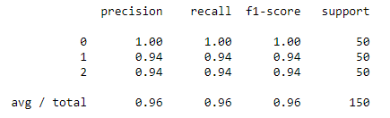
accuracy = getAccuracy(testSet, predictions)
print('Accuracy: ' + repr(accuracy) + '%')
main()
This was all about the kNN Algorithm using python. In case you are still left with a query, don’t hesitate in adding your doubt to the blog’s comment section.

Machine Learning with R Machine learning is the present and the future! From Netflix’s recommendation engine to Google’s self-driving car, it’s all machine learning. This blog on Machine Learning with R helps you understand the core concepts of machine learning followed by different machine learning algorithms and implementing those machine learning algorithms with R. This […]

Most football enthusiasts will know that the sport has been a bit slower than others when it comes to adopting new technologies. There are several speculated reasons for this — the game’s age and the fact that it is dominated by traditionalists — to name a few. Nevertheless, this year’s football world cup seems to […]

Tennis is a wonderful and unique sport, no doubt about it. What makes tennis unique is not the interesting gameplay it offers or the massive following it commands, this racket-ball sport is one-of-its-kind because of the speed at which it adopts new-age technologies, such as AI in Wimbledon this year. To ensure that the sport […]

Football is arguably the most popular sport in the world. According to FIFA.com, a total of 3.2 billion people tuned in to watch the 2014 football World Cup. But, did you know that technology is playing a crucial role in making football what it is today? In fact, modern football can be considered an autonomous […]

Unlike most domains, Information Technology is dynamic and changes rapidly in short periods of time. If you are a technology professional, it is very important to re-skill yourself to survive in this highly competitive IT industry. For instance, let’s look at the curious case of a Java developer. A decade ago, Java professionals were a […]


AI vs Machine Learning vs Deep Learning, these terms have confused a lot of people. If you too are one among them then this blog – AI vs Machine Learning vs Deep Learning is definitely for you. AI vs Machine Learning vs Deep Learning Artificial Intelligence is the broader umbrella under which Machine Learning and Deep […]

Machine learning has gone through many recent developments and is becoming more popular day by day. Machine Learning is being used in various projects to find hidden information in data by people from all domains, including Computer Science, Mathematics, and Management. It was just a matter of time that Apache Spark Jumped into the game of Machine […]
The post K-Nearest Neighbors Algorithm Using Python appeared first on Edureka Blog.


 In the Build tab, click on invoke top level maven targets and use the below command:


 DevOps is a software development approach which involves continuous development, continuous testing, continuous integration, continuous deployment and continuous monitoring of the software throughout its development life cycle. This is exactly the process adopted by all the top companies to develop high-quality software and shorter development life cycles, resulting in greater customer satisfaction, something that every company wants.
 The above pipeline is a logical demonstration of how a software will move along the various phases or stages in this lifecycle, before it is delivered to the customer or before it is live on production.
  Suppose we have a Java code and it needs to be compiled before execution. So, through the version control phase, it again goes to build phase where it gets compiled. You get all the features of that code from various branches of the repository, which merge them and finally use a compiler to compile it. This whole process is called the build phase.
 Once the build phase is over, then you move on to the testing phase. In this phase, we have various kinds of testing, one of them is the unit test (where you test the chunk/unit of software or for its sanity test).
 When the test is completed, you move on to the deploy phase, where you deploy it into a staging or a test server. Here, you can view the code or you can view the app in a simulator.


 Jenkins provides us with various interfaces and tools in order to automate the entire process


 Now you might be wondering about its working. Well, the data in an RDD is split into chunks based on a key. RDDs are highly resilient, i.e, they are able to recover quickly from any issues as the same data chunks are replicated across multiple executor nodes. Thus, even if one executor node fails, another will still process the data. This allows you to perform your functional calculations against your dataset very quickly by harnessing the power of multiple nodes.
  Moreover, once you create an RDD it becomes


 Using ReduceByKey transformation to reduce the data


 Most organisations use behavioural analytics of customers in order to provide customer satisfaction and hence, increase their customer base. The best example of this is Amazon. Amazon is one of the best and most widely used e-commerce websites with a customer base of about 300 million. They use customer click-stream data and historical purchase data to provide them with customized results on customized web pages.
 Big data technologies and technological advancements like cloud computing bring significant cost advantages when it comes to store and process Big Data. Let me tell you how healthcare utilizes Big Data Analytics to reduce their costs. Patients nowadays are using new sensor devices when at home or outside, which send constant streams of data that can be monitored and analysed in real-time to help patients avoid hospitalization by self-managing their conditions.


 Written on Golang, it has a huge community because it was first developed by Google & later donated to CNCF
 Kubernetes Architecture has the following main components:
 It is the entry point for all administrative tasks which is responsible for managing the Kubernetes cluster. There can be more than one master node in the cluster to check for fault tolerance. More than one master node puts the system in a High Availability mode, in which one of them will be the main node which we perform all the tasks.
 It is a physical server or you can say a VM which runs the applications using Pods (a pod scheduling unit) which is controlled by the master node. On a physical server (worker/slave node), pods are scheduled. For accessing
  They used a
  With the Deployer in place,


